Generalized Logistic Analysis

This function implements the generalized logistic analysis introduced in Verboon & Peters (2017). This analysis fits a logistic function (i.e. a sigmoid) to a data series. This is useful when analysing single case designs. The function enables easy customization of the main plot elements and easy saving of the plot with anti-aliasing. ggGenLogPlot does most of the plotting, and can be useful when trying to figure out sensible starting and boundary/constraint values. genlogCompleteStartValues tries to compute sensible starting and boundary/constraint values based on the data.

genlog(data,
       timeVar = 1,
       yVar = 2,
       phaseVar = NULL,
       baselineMeasurements = NULL,
       yRange = NULL,
       startX = NULL,
       startBase = NULL,
       startTop = NULL,
       startGrowthRate = NULL,
       startV = 1,
       changeInitiationBounds = NULL,
       growthRateBounds = c(-2, 2),
       baseMargin = c(0, 3),
       topMargin = c(-3, 0),
       baseBounds = NULL,
       topBounds = NULL,
       vBounds = c(1, 1),
       colors = list(bounds = viridis(4)[4],
                     curve = viridis(4)[3],
                     mid = viridis(4)[2],
                     intervention = viridis(4)[1],
                     points = "black"),
       alphas = list(outsideRange = .2,
                     bounds = 0,
                     points = .5,
                     mid = 0),
       theme = theme_minimal(),
       pointSize = 2,
       pointAlpha = 0.5,
       lineSize = 0.5,
       initialValuesLineType = "blank",
       curveSizeMultiplier = 2,
       showPlot = TRUE,
       plotLabs = NULL,
       outputFile = NULL,
       outputWidth = 16,
       outputHeight = 16,
       ggsaveParams = list(units = "cm",
                           dpi = 300,
                           type = "cairo"))

Arguments

data	The dataframe containing the variables for the analysis.
timeVar	The name of the variable containing the measurement moments (or an index of measurement moments). An index can also be specified, and assumed to be 1 if omitted.
yVar	The name of the dependent variable. An index can also be specified, and assumed to be 2 if omitted.
phaseVar	The variable containing the phase of each measurement. Note that this normally should only have two possible values.
baselineMeasurements	If no phaseVar is specified, baselineMeasurements can be used to specify the number of baseline measurements, which is then used to construct the phaseVar dummy variable.
yRange	This can be used to manually specify the possible values that the dependent variable can take. If no startBase and startTop are specified, the range of the dependent variable is used instead.
startX, startBase, startTop, startGrowthRate, startV	The starting values used when estimating the sigmoid using minpack.lm's nlsLM function. startX specifies the starting value to use for the measurement moment when the change is fastest (i.e. the slope of the sigmoid has the largest value); startBase and startTop specify the starting values to use for the base (floor) and top (ceiling), the plateaus of relative stability between which the sigmoid described the shift; startGrowthRate specifies the starting value for the growth rate; and startV specifies the starting value for the v parameter.
changeInitiationBounds, growthRateBounds, baseMargin, topMargin, baseBounds, topBounds, vBounds	These values specify constraints to respect when estimating the parameters of the sigmoid function using minpack.lm's nlsLM. changeInitiationBounds specifies between which values the initiation of the shift must occur; growthRateBounds describes the bounds constraining the possible values for the growth rate; baseBounds and topBounds specify the constraints for possible values for the base (floor) and top (ceiling), the plateaus of relative stability between which the sigmoid described the shift; and if these are not specified, baseMargin and topMargin are used in combination with the range of the dependent variable to set these bounds (also see yRange); and finally, vBounds specifies the possible values that constrain the v parameter.
colors	The colors to use for the different plot elements.
alpha	The alpha values (transparency, or rather, 'obliqueness', with 0 indicating full transparency and 1 indicating full visibility) to use for the different plot elements.
theme	The theme to use in the plot.
pointSize,lineSize	The sizes of points and lines in the plot.
pointAlpha	The alpha channel (transparency, or rather, 'opaqueness') of the points.
initialValuesLineType	The line type to use for the initial values; by default set to "blank" for genlog, to hide them, and to "dashed" for ggGenLogPlot.
curveSizeMultiplier	A multiplyer for the curve size compared to the other lines (e.g. specify '2' to have a curve of twice the size).
showPlot	Whether to show the plot or not.
plotLabs	A list with arguments to the ggplot2 labs function, which can be used to conveniently set plot labels.
outputFile	If not NULL, the path and filename specifying where to save the plot.
outputWidth, outputHeight	The dimensions of the plot when saving it (in units specified in ggsaveParams).
ggsaveParams	The parameters to use when saving the plot, passed on to ggsave.

Details

For details, see Verboon & Peters (2017).

Value

Mainly, this function prints its results, but it also returns them in an object containing three lists:

input

The arguments specified when calling the function

intermediate

Intermediat objects and values

output

The results such as the plot.

References

Verboon, P. & Peters, G.-J. Y. (2018) Applying the generalised logistic model in single case designs: modelling treatment-induced shifts. PsyArXiv https://doi.org/10.17605/osf.io/ad5eh

See also

genlogFunction

Examples

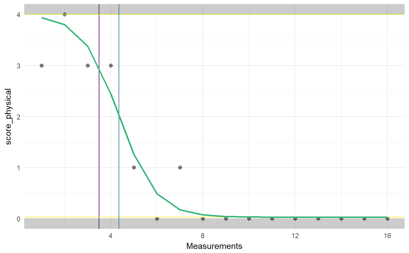
### Load dataset
data(Singh);

### Extract Jason
dat <- Singh[Singh$tier==1, ];

### Conduct piecewise regression analysis
genlog(dat,
       timeVar='time',
       yVar='score_physical',
       phaseVar='phase');
#> Generalized Logistic Analysis (N = 16)
#> 
#> Estimated sigmoid association between time and score_physical.
#> 
#> Parameter starting values [and constraints]:
#>   Onset of change: 7* [2; 12]*
#>   Curve base:      0* [0; 3]*
#>   Growth rate:     0* [-2; 2]
#>   Curve top:       4* [1; 4]*
#>   V parameter:     1 [1; 1]
#> 
#> Note: Asterisks (*) denote values that were not specified manually (but inferred by genlog).
#> 
#> Parameter estimates:
#> 
#>   Curve base (plateau before change): 0.031
#>   Growth rate:                        -1.241
#>   Change maximal at:                  4.355
#>   Curve top (plateau after change):   4
#> 
#> Model fit and effect sizes estimates:
#> 
#>   Deviance:          2.374
#>   R squared:         0.923
#>   Effect Size 1:     2.764
#>   Effect Size 2:     0.992