Flexible anova

This function is meant as a userfriendly wrapper to approximate the way analysis of variance is done in SPSS.

fanova(data,
       y,
       between = NULL,
       covar = NULL,
       plot = FALSE,
       levene = FALSE,
       digits = 2,
       contrast = NULL)

Arguments

data	The dataset containing the variables to analyse.
y	The dependent variable. For oneway anova, factorial anova, or ancova, this is the name of a variable in dataframe data. For repeated measures anova, this is a vector with the names of all variable names in dataframe data, e.g. c('t0_value', 't1_value', 't2_value').
between	A vector with the variables name(s) of the between subjects factor(s).
covar	A vector with the variables name(s) of the covariate(s).
plot	Whether to produce a plot. Note that a plot is only produced for oneway and twoway anova and oneway repeated measures designs: if covariates or more than two between-subjects factors are specified, not plot is produced. For twoway anova designs, the second predictor is plotted as moderator (and the first predictor is plotted on the x axis).
levene	Whether to show Levene's test for equality of variances (using car's leveneTest function but specifying mean as function to compute the center of each group).
digits	Number of digits (actually: decimals) to use when printing results. The p-value is printed with one extra digit.
contrast	This functionality has not been implemented yet.

Details

This wrapper uses oneway and lm and lmer in combination with car's Anova function to conduct the analysis of variance.

Value

Mainly, this function prints its results, but it also returns them in an object containing three lists:

input

The arguments specified when calling the function

intermediate

Intermediat objects and values

output

The results such as the plot.

See also

regr and logRegr for similar functions for linear and logistic regression and oneway, lm, lmer and Anova for the functions used behind the scenes.

Examples

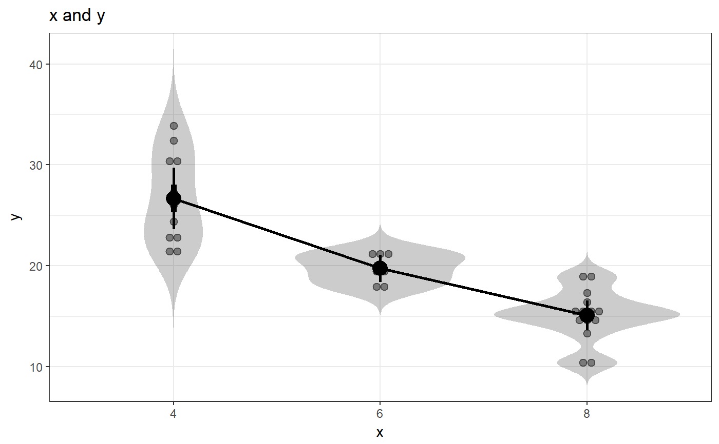
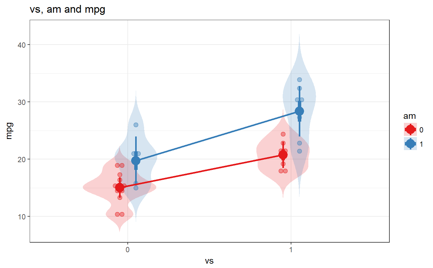
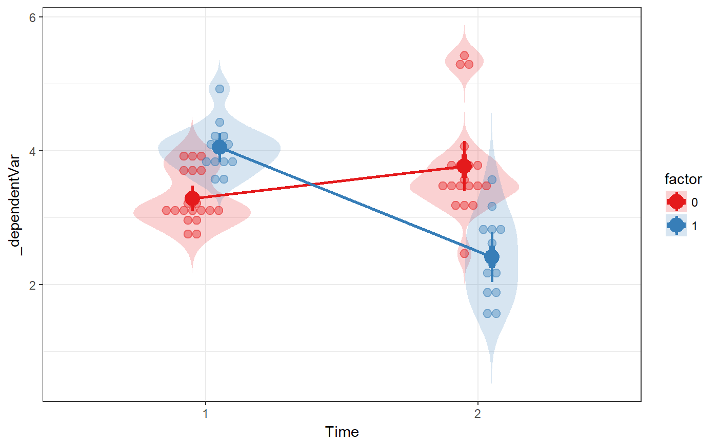
### Oneway anova with a plot
fanova(dat=mtcars, y='mpg', between='cyl', plot=TRUE);
#> Flexible Analysis of Variance was called with:
#> 
#>   Dependent variable: mpg
#>   Factors: cyl
#> 
#> Between-subjects factor 'cyl' does not have class 'factor' in dataframe 'mtcars'. Converting it now.
#> 
#> ### Oneway Anova for y=y and x=x (groups: 4, 6, 8)
#> 
#> Omega squared: 95% CI = [.51; .81], point estimate = .71
#> Eta Squared: 95% CI = [.55; .8], point estimate = .73
#> 
#>                                     SS Df     MS    F     p
#> Between groups (error + effect) 824.78  2 412.39 39.7 <.001
#> Within groups (error only)      301.26 29  10.39           
#> 

### Factorial anova
fanova(dat=mtcars, y='mpg', between=c('vs', 'am'), plot=TRUE);
#> Flexible Analysis of Variance was called with:
#> 
#>   Dependent variable: mpg
#>   Factors: vs & am
#> 
#> Between-subjects factor 'vs' does not have class 'factor' in dataframe 'mtcars'. Converting it now.
#> Between-subjects factor 'am' does not have class 'factor' in dataframe 'mtcars'. Converting it now.
#> 
#> Anova Table (Type III tests)
#> 
#> Response: mpg
#>              Sum Sq Df  F value    Pr(>F)    
#> (Intercept) 2718.03  1 225.5116 6.344e-15 ***
#> vs           143.28  1  11.8878  0.001805 ** 
#> am            88.36  1   7.3311  0.011420 *  
#> vs:am         16.01  1   1.3283  0.258855    
#> Residuals    337.48 28                       
#> ---
#> Signif. codes:  0 ‘***’ 0.001 ‘**’ 0.01 ‘*’ 0.05 ‘.’ 0.1 ‘ ’ 1

### Ancova
fanova(dat=mtcars, y='mpg', between=c('vs', 'am'), covar='hp');
#> Flexible Analysis of Variance was called with:
#> 
#>   Dependent variable: mpg
#>   Factors: vs & am
#>   Covariates: hp
#> 
#> Between-subjects factor 'vs' does not have class 'factor' in dataframe 'mtcars'. Converting it now.
#> Between-subjects factor 'am' does not have class 'factor' in dataframe 'mtcars'. Converting it now.
#> 
#> Anova Table (Type III tests)
#> 
#> Response: mpg
#>              Sum Sq Df F value    Pr(>F)    
#> (Intercept) 170.670  1 22.7259 7.507e-05 ***
#> vs            8.072  1  1.0748    0.3102    
#> am            2.527  1  0.3365    0.5673    
#> hp           21.750  1  2.8962    0.1017    
#> vs:am         1.045  1  0.1392    0.7123    
#> vs:hp         7.096  1  0.9449    0.3407    
#> am:hp         0.275  1  0.0366    0.8498    
#> vs:am:hp      0.378  1  0.0503    0.8244    
#> Residuals   180.238 24                      
#> ---
#> Signif. codes:  0 ‘***’ 0.001 ‘**’ 0.01 ‘*’ 0.05 ‘.’ 0.1 ‘ ’ 1

### Repeated measures anova; first generate datafile
dat <- mtcars[, c('am', 'drat', 'wt')];
names(dat) <- c('factor', 't0_dependentVar' ,'t1_dependentVar');
dat$factor <- factor(dat$factor);

### Then do the repeated measures anova
fanova(dat, y=c('t0_dependentVar' ,'t1_dependentVar'),
       between='factor', plot=TRUE);
#> Flexible Analysis of Variance was called with:
#> 
#>   Dependent variable: _dependentVar
#>   Factors: factor
#> 
#> 
#> Analysis of Deviance Table (Type III Wald F tests with Kenward-Roger df)
#> 
#> Response: y
#>                    F Df Df.res    Pr(>F)    
#> (Intercept) 291.1299  1 273.52 < 2.2e-16 ***
#> factor       13.6367  1  60.00 0.0004811 ***
#> time          3.1389  1 273.52 0.0775596 .  
#> factor:time  52.6222  1  60.00 9.214e-10 ***
#> ---
#> Signif. codes:  0 ‘***’ 0.001 ‘**’ 0.01 ‘*’ 0.05 ‘.’ 0.1 ‘ ’ 1