Userfriendly wrapper to do logistic regression in R

This function is meant as a userfriendly wrapper to approximate the way logistic regression is done in SPSS.

logRegr(formula,
        data = NULL,
        conf.level = 0.95,
        digits = 2,
        pvalueDigits = 3,
        crossTabs = TRUE,
        plot = FALSE,
        collinearity = FALSE,
        env = parent.frame(),
        predictionColor = viridis(3)[3],
        predictionAlpha = 0.5,
        predictionSize = 2,
        dataColor = viridis(3)[1],
        dataAlpha = 0.33,
        dataSize = 2,
        observedMeansColor = viridis(3)[2],
        binObservedMeans = 7,
        observedMeansSize = 2,
        observedMeansWidth = NULL,
        observedMeansAlpha = 0.5,
        theme = theme_bw())

Arguments

formula	The formula, specified in the same way as for glm (which is used for the actual analysis).
data	Optionally, a dataset containing the variables in the formula (if not specified, the variables must exist in the environment specified in env.
conf.level	The confidence level for the confidence intervals.
digits	The number of digits used when printing the results.
pvalueDigits	The number of digits used when printing the p-values.
crossTabs	Whether to show cross tabulations of the correct predictions for the null model and the tested model, as well as the percentage of correct predictions.
plot	Whether to display the plot.
collinearity	Whether to show collinearity diagnostics.
env	If no dataframe is specified in data, use this argument to specify the environment holding the variables in the formula.
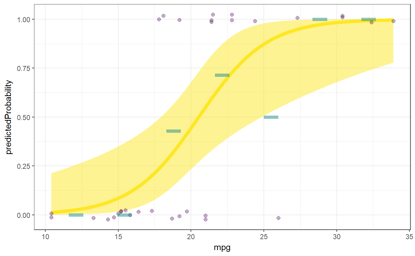
predictionColor, dataColor, observedMeansColor	The color of, respectively, the line and confidence interval showing the prediction; the points representing the observed data points; and the means based on the observed data.
predictionAlpha, dataAlpha, observedMeansAlpha	The alpha of, respectively, the confidence interval of the prediction; the points representing the observed data points; and the means based on the observed data (set to 0 to hide an element).
predictionSize, dataSize, observedMeansSize	The size of, respectively, the line of the prediction; the points representing the observed data points; and the means based on the observed data (set to 0 to hide an element).
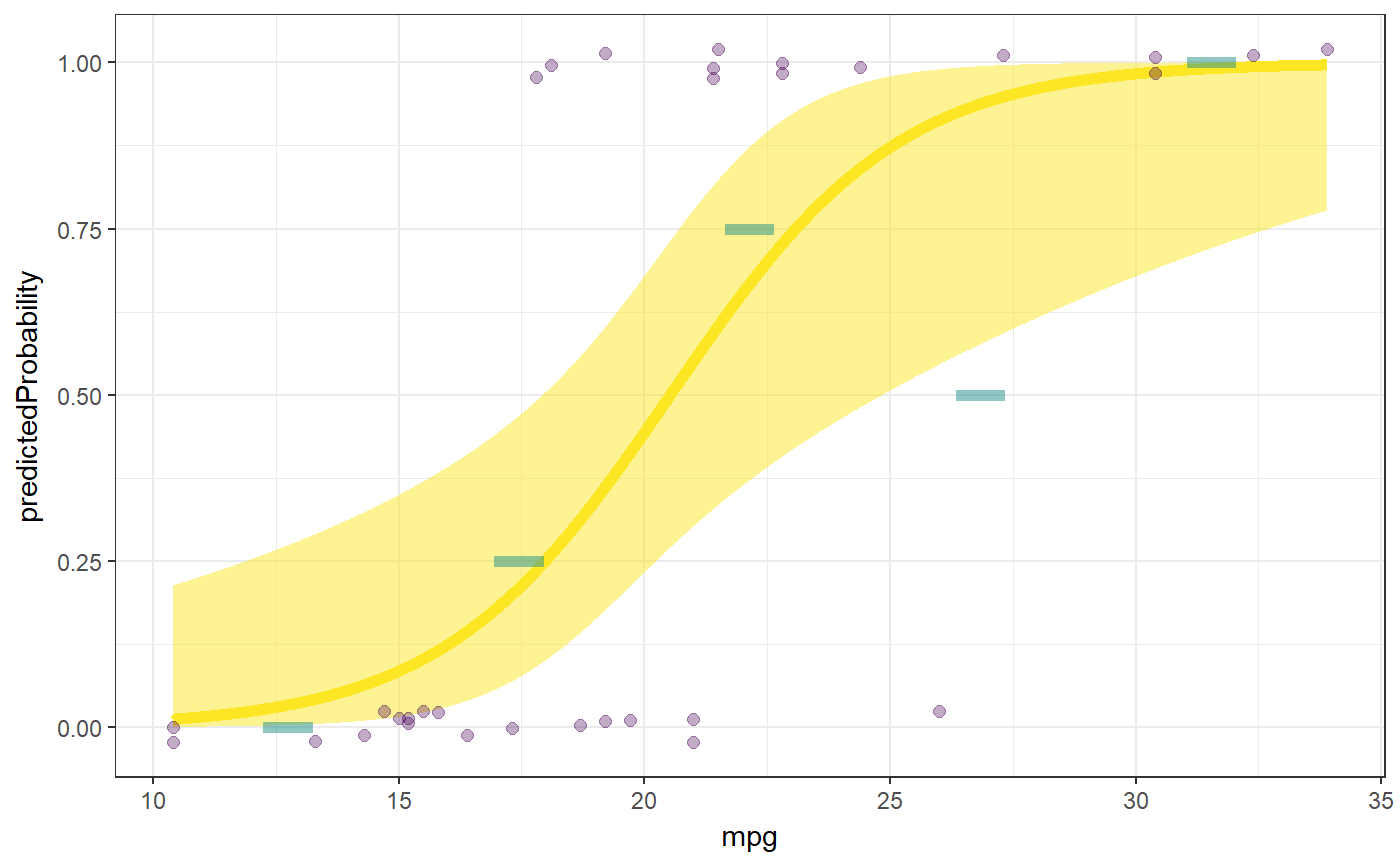
binObservedMeans	Whether to bin the observed means; either FALSE or a single numeric value specifying the number of bins.
observedMeansWidth	The width of the lines of the observed means. If not specified (i.e. NULL), this is computed automatically and set to the length of the shortest interval between two successive points in the predictor data series (found using findShortestInterval.
theme	The theme used to display the plot.

Details

This function

Value

Mainly, this function prints its results, but it also returns them in an object containing three lists:

input

The arguments specified when calling the function

intermediate

Intermediat objects and values

output

The results, such as the plot, the cross tables, and the coefficients.

See also

regr and fanova for similar functions for linear regression and analysis of variance and glm for the regular interface for logistic regression.

Examples

### Simplest way to call logRegr
logRegr(data=mtcars, formula = vs ~ mpg);
#> Waiting for profiling to be done...
#> Logistic regression analysis for formula: vs ~ mpg
#> 
#> Significance test of the entire model (all predictors together):
#>   Cox & Snell R-squared: 0.44,
#>   Nagelkerke R-squared: 0.58
#>   Test for significance: ChiSq[1] = 18.33, p < .001
#> 
#> Predictions by the null model (56.25% correct):
#> 
#>         Predicted
#> Observed  0
#>        0 18
#>        1 14
#> 
#> Predictions by the tested model (81.25% correct):
#> 
#>         Predicted
#> Observed  0  1
#>        0 15  3
#>        1  3 11
#> 
#> Raw regression coefficients (log odds values, called 'B' in SPSS):
#> 
#>             95% conf. int. estimate   se     z    p
#> (Intercept) [-16.74; -3.9]    -8.83 3.16 -2.79 .005
#> mpg           [0.18; 0.82]     0.43 0.16  2.72 .007
#> 

### Also ordering a plot
logRegr(data=mtcars, formula = vs ~ mpg, plot=TRUE);
#> Waiting for profiling to be done...
#> Logistic regression analysis for formula: vs ~ mpg
#> 
#> Significance test of the entire model (all predictors together):
#>   Cox & Snell R-squared: 0.44,
#>   Nagelkerke R-squared: 0.58
#>   Test for significance: ChiSq[1] = 18.33, p < .001
#> 
#> Predictions by the null model (56.25% correct):
#> 
#>         Predicted
#> Observed  0
#>        0 18
#>        1 14
#> 
#> Predictions by the tested model (81.25% correct):
#> 
#>         Predicted
#> Observed  0  1
#>        0 15  3
#>        1  3 11
#> 
#> Raw regression coefficients (log odds values, called 'B' in SPSS):
#> 
#>             95% conf. int. estimate   se     z    p
#> (Intercept) [-16.74; -3.9]    -8.83 3.16 -2.79 .005
#> mpg           [0.18; 0.82]     0.43 0.16  2.72 .007
#> 

### Only use five bins
logRegr(data=mtcars, formula = vs ~ mpg, plot=TRUE, binObservedMeans=5);
#> Waiting for profiling to be done...
#> Logistic regression analysis for formula: vs ~ mpg
#> 
#> Significance test of the entire model (all predictors together):
#>   Cox & Snell R-squared: 0.44,
#>   Nagelkerke R-squared: 0.58
#>   Test for significance: ChiSq[1] = 18.33, p < .001
#> 
#> Predictions by the null model (56.25% correct):
#> 
#>         Predicted
#> Observed  0
#>        0 18
#>        1 14
#> 
#> Predictions by the tested model (81.25% correct):
#> 
#>         Predicted
#> Observed  0  1
#>        0 15  3
#>        1  3 11
#> 
#> Raw regression coefficients (log odds values, called 'B' in SPSS):
#> 
#>             95% conf. int. estimate   se     z    p
#> (Intercept) [-16.74; -3.9]    -8.83 3.16 -2.79 .005
#> mpg           [0.18; 0.82]     0.43 0.16  2.72 .007
#>