Piecewise regression analysis

This function conducts a piecewise regression analysis and shows a plot illustrating the results. The function enables easy customization of the main plot elements and easy saving of the plot with anti-aliasing.

piecewiseRegr(data,
              timeVar = 1,
              yVar = 2,
              phaseVar = NULL,
              baselineMeasurements = NULL,
              robust = FALSE,
              digits = 2,
              colors = list(pre = viridis(4)[1],
                            post = viridis(4)[4],
                            diff = viridis(4)[3],
                            intervention = viridis(4)[2],
                            points = "black"),
              theme = theme_minimal(),
              pointSize = 2,
              pointAlpha = 1,
              lineSize = 1,
              showPlot = TRUE,
              plotLabs = NULL,
              outputFile = NULL,
              outputWidth = 16,
              outputHeight = 16,
              ggsaveParams = list(units = "cm",
                                  dpi = 300,
                                  type = "cairo"))

Arguments

data	The dataframe containing the variables for the analysis.
timeVar	The name of the variable containing the measurement moments (or an index of measurement moments). An index can also be specified, and assumed to be 1 if omitted.
yVar	The name of the dependent variable. An index can also be specified, and assumed to be 2 if omitted.
phaseVar	The variable containing the phase of each measurement. Note that this normally should only have two possible values.
baselineMeasurements	If no phaseVar is specified, baselineMeasurements can be used to specify the number of baseline measurements, which is then used to construct the phaseVar dummy variable.
robust	Whether to use normal or robust linear regression.
digits	The number of digits to show in the results.
colors	The colors to use for the different plot elements.
theme	The theme to use in the plot.
pointSize,lineSize	The sizes of points and lines in the plot.
pointAlpha	The alpha channel (transparency, or rather, 'opaqueness') of the points.
showPlot	Whether to show the plot or not.
plotLabs	A list with arguments to the ggplot2 labs function, which can be used to conveniently set plot labels.
outputFile	If not NULL, the path and filename specifying where to save the plot.
outputWidth, outputHeight	The dimensions of the plot when saving it (in units specified in ggsaveParams).
ggsaveParams	The parameters to use when saving the plot, passed on to ggsave.

Value

Mainly, this function prints its results, but it also returns them in an object containing three lists:

input

The arguments specified when calling the function

intermediate

Intermediat objects and values

output

The results such as the plot.

References

Verboon, P. & Peters, G.-J. Y. (2018) Applying the generalised logistic model in single case designs: modelling treatment-induced shifts. PsyArXiv https://doi.org/10.17605/osf.io/ad5eh

See also

genlog

Examples

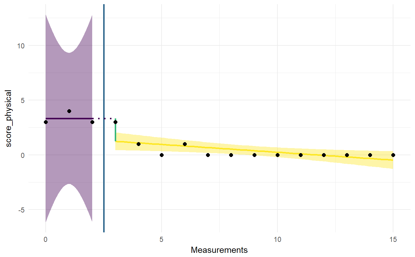
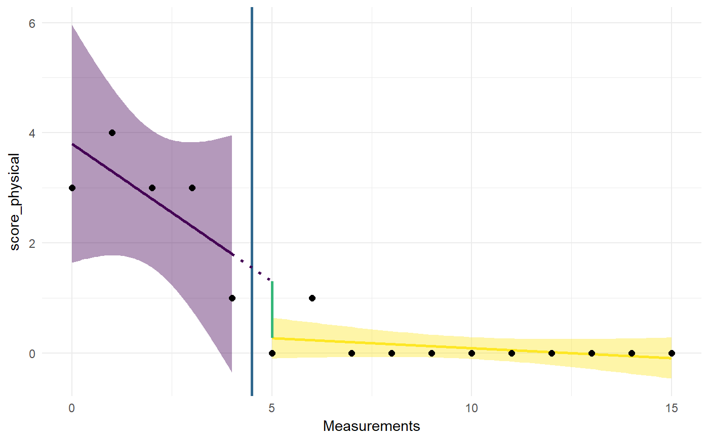
### Load dataset
data(Singh);

### Extract Jason
dat <- Singh[Singh$tier==1, ];

### Conduct piecewise regression analysis
piecewiseRegr(dat,
              timeVar='time',
              yVar='score_physical',
              phaseVar='phase');
#> Piecewise Regression Analysis (N = 16)
#> 
#> Model statistics:
#> 
#>   Model deviance:              6.03
#>   R squared for null model:    .66
#>   R squared for test model:    .81
#>   R squared based effect size: .42
#> 
#> Regression coefficients:
#> 
#>   Intercept:        [1.92; 4.74] (point estimate = 3.33)
#>   Level change:     [-4.59; 0.4] (point estimate = -2.09)
#>   Trend phase 1:   [-1.09; 1.09] (point estimate = 0)
#>   Change in trend: [-1.24; 0.96] (point estimate = -0.14)

### Pretend treatment started between measurements
### 5 and 6
piecewiseRegr(dat,
              timeVar='time',
              yVar='score_physical',
              baselineMeasurements=5);
#> Piecewise Regression Analysis (N = 16)
#> 
#> Model statistics:
#> 
#>   Model deviance:              3.06
#>   R squared for null model:    .66
#>   R squared for test model:    .9
#>   R squared based effect size: .71
#> 
#> Regression coefficients:
#> 
#>   Intercept:         [2.95; 4.65] (point estimate = 3.8)
#>   Level change:     [-2.34; 0.28] (point estimate = -1.03)
#>   Trend phase 1:   [-0.85; -0.15] (point estimate = -0.5)
#>   Change in trend:    [0.1; 0.83] (point estimate = 0.46)